Authors & affiliations

Ritwika Das and Javiera Cartagena-Farias, Care Policy and Evaluation Centre, London School of Economics and Political Science

 

Introduction

Regression Discontinuity Design (RDD) is a quasi-experimental method that exploits threshold-based policy rules to estimate causal effects (Thistlethwaite & Campbell, 1960). The basic idea is simple: when access to a programme or intervention is determined by a threshold, people just above and just below that cut-off are likely to be very similar. This makes it possible to compare them in a way that approximates a randomised experiment. When treatment is assigned based on a clear rule, RDD offers a practical and credible way to assess impact. While this methodology has been more widely used in education and welfare-related research, its application in health care and long-term care settings has been limited so far (Venkataramani, Bor & Jena, 2016).

 

Description

RDD is easiest to understand when we think about a simple yes-or-no treatment. Imagine there is a rule: if you score above a certain threshold (e.g. you are above certain age), you receive a treatment; if you score below it, you do not. The variable (X) that determines this is called the running variable (or forcing variable). X perfectly determines treatment status as a function of a cut-off point c. All this can be formally written down as follows:

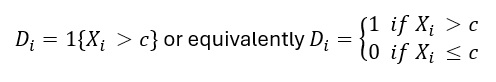
If a person’s score on the running variable is above the cut-off point , then  (they receive the treatment). If their score is at or below the cut-off, then  (they do not receive the treatment). The treatment can be the participation in a fall’s prevention programme, a cash transfer for unpaid carers, etc. In practice, when performing RDD, usually not everyone in the dataset is used for analysis. Instead, the focus is on individuals who are close to the cut-off, since these are the most comparable. To do this, a bandwidth is defined, often denoted by . The bandwidth determines how wide the “window” is around the cut-off and therefore which observations are included in the analysis (Angrist & Pischke, 2008).  See Figure 1 for a visual illustration:

 

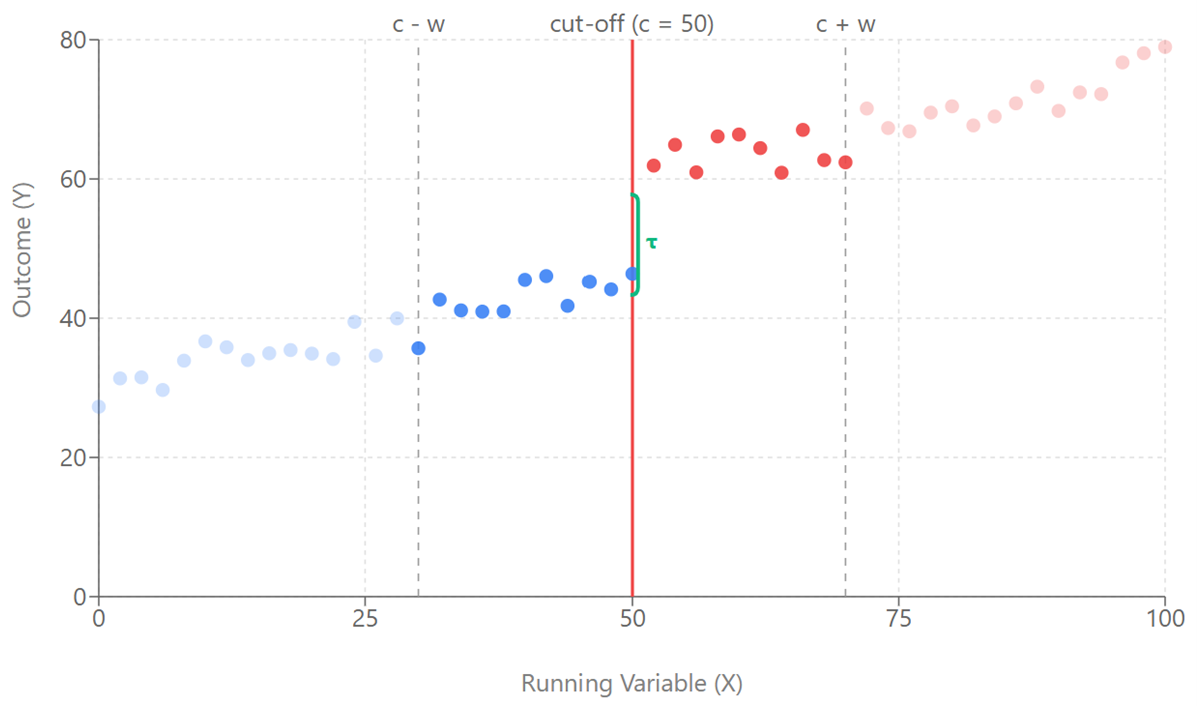
Figure 1: The vertical distance between the two trend lines at the cut-off represents the treatment effect. Points within the bandwidth (darker) are used for estimation, while those outside (lighter) are excluded from the analysis.

 

RDD comes in two main forms: sharp RDD and fuzzy RDD. In sharp RDD, the cut-off perfectly determines who gets treated i.e. if an individual falls above the cut-off, they receive treatment and if they fall below it, they do not receive treatment. On the other hand, fuzzy RDD does not rigidly determine treatment assignment. In this variation, some individuals just above the cut-off may not get treated, while some just below it may still receive treatment. This makes the treatment assignment probabilistic rather than deterministic as seen in the case of sharp RDD (Cattaneo, 2020).

 

Bandwidth, Kernel, and polynomial order

To estimate the treatment effect, a few decisions need to be taken. The first is about the bandwidth (w). The bandwidth defines how close to the threshold observations must be in order to be compared (Cattaneo et al. 2020).

• A narrower bandwidth focuses only on units very close to the cut-off. This makes the local randomisation assumption more credible, since individuals just above and below the threshold are likely to be very similar. However, using fewer observations reduces statistical power and may increase uncertainty.
• A wider bandwidth includes more observations, improving precision, but it risks comparing individuals who are less similar, which may introduce bias.

To balance this trade-off between bias and variance, researchers often rely on the Imbens-Kalyanaraman (2012) method or the Calonico-Cattaneo-Titiunik (2014) robust bias-corrected approach.

Another important choice is the kernel function. The kernel determines how much weight is given to observations depending on their distance from the cut-off. In theory, more weight should be given to observations that are closer to the threshold, since these are the most comparable. Common kernel choices include:

• Uniform kernel: gives equal weight to all observations within the bandwidth.
• Triangular kernel: gives more weight to observations closer to the cut-off and less weight to those further away.
• Epanechnikov kernel: uses a curved weighting scheme that gradually reduces weights with distance.

The triangular kernel is generally preferred in applied work because it places the greatest emphasis on observations nearest the cut-off. Deviating from it typically requires a clear justification.

Another important choice is the polynomial order (p). This determines the type of curve we fit to the data on each side of the cut-off. For example:

• If p = 1, we fit a local linear regression, meaning we approximate the relationship using straight lines near the cut-off.
• If p = 2, we fit a local quadratic regression, which allows for some curvature.

Higher-order polynomials can capture more complex patterns in the data. However, they can also lead to overfitting and unstable estimates, particularly near the boundaries of the data. For this reason, most researchers recommend using local linear regression (p = 1), as it is simpler and tends to be more robust. Local quadratic models are sometimes used as a robustness check.

Finally, it is good practice to conduct sensitivity analyses. This means re-estimating the treatment effect using different bandwidths, polynomial orders, or kernel choices to check whether the results remain stable across specifications (Cattaneo et al., 2024). If the estimated effect changes substantially with small adjustments, this may indicate that the results are not robust.

In R and Stata, RDD is implemented as follows:

In R, using the rdrobust package:

library(rdrobust)
rdrobust(y = y,
x = x,
c = cutoff,
h = 5,
p = 1,
kernel = “triangular”)

 

In Stata, using the rdrobust command:

rdrobust y x, c(cutoff) h(5) p(1) kernel(triangular)

 

Strengths & Limitations

RDD is an attractive method for causal identification because it relies on fewer assumptions than other approaches. For instance, methods such as Propensity Score Matching assume that, once we control for observed characteristics, treatment assignment is effectively random. In other words, they require that there are no unobserved differences affecting both treatment and outcomes. RDD does not rely on this assumption. Instead, it focuses on individuals who are very close to the cut-off point. Around this threshold, people are likely to be very similar to one another, except for whether they just qualified for the treatment or just missed it. This local comparison allows us to estimate causal effects without needing to assume that treatment assignment is independent of potential outcomes conditional on observed characteristics. This means individuals can differ in unobserved ways, as long as the assignment rule at the cut-off is followed.

RDD also does not assume that treatment effects are the same for everyone (i.e. homogenous treatment effects). Instead, it estimates a Local Average Treatment Effect at the cut-off. In other words, it tells us the effect of the treatment for individuals who are just eligible compared with those who just miss eligibility. Effects may differ elsewhere, and that does not invalidate the design.

That said, RDD does rely on some important assumptions. First, individuals must not be able to precisely manipulate their position relative to the cut-off. Second, in the absence of treatment, potential outcomes should change smoothly at the threshold. In addition, other characteristics should be balanced and continuous around the cut-off.

Overall, RDD remains a robust method because it requires relatively weak assumptions about global relationships across the data, while placing strong and testable requirements on behaviour close to the threshold.

 

Further Extensions

Beyond the traditional RDD we can find:

• Regression kink designs (RKD) identify causal effects when the relationship between the running variable and treatment intensity changes slope at a known cut-off. The treatment effect for RKD is therefore popularly known as Local Average Response (LAR). For example, if a policy assigns benefits that increase linearly with income up to a certain threshold and then increase at a different rate beyond that point, the “kink” in this relationship creates identification.
• Geographic (Spatial) RDD. Cut-off is based on location (e.g., distance to care services).

 

Example (in long-term care)

Some applications of the RDD approach to long-term care research include the following:

• Cartagena-Farias, Brimblecombe & Knapp (2024) evaluated the association between receipt of a winter fuel cash transfer and older people’s care needs, quality of life, and housing quality in England, using a sharp RDD.
• Wang, et al. (2024) explored the effect of retirement on physical and mental health in China performing a fuzzy RDD.
• Menezes-Filho & Politi (2020) estimated the causal effects of private health insurance in Brazil using a regression kink design.

 

References

References

Angrist, J. D., & Pischke, J. S. (2008). Mostly harmless econometrics. Princeton University Press.

Calonico, S., Cattaneo, M. D., & Titiunik, R. (2014). Robust nonparametric confidence intervals for regression-discontinuity designs. Econometrica, 82(6), 2295–2326. https://doi.org/10.3982/ECTA11757

Calonico, S., Cattaneo, Matias D., Max H. Farrell. (2020). “Optimal bandwidth choice for robust bias-corrected inference in regression discontinuity designs.” The Econometrics Journal, 23(2), 192–210. DOI: 10.1093/ectj/utz022

Cartagena-Farias, J., Brimblecombe, N., & Knapp, M. (2024). Evaluating the association between receipt of a winter fuel cash transfer and older people’s care needs, quality of life, and housing quality: Evidence from England. Social Science & Medicine, 355, 117128. DOI: 10.1016/j.socscimed.2024.117128

Cattaneo, Matias D., Richard K. Crump, Max H. Farrell, and Yingjie Feng. (2024). “On Binscatter.” American Economic Review, 114(5), 1488–1514. DOI: 10.1257/aer.20221576

Imbens, G. W., & Kalyanaraman, K. (2012). Optimal bandwidth choice for the regression discontinuity estimator. The Review of Economic Studies, 79(3), 933–959.

Menezes-Filho, N., & Politi, R. (2020). Estimating the causal effects of private health insurance in Brazil: Evidence from a regression kink design. Social Science & Medicine, 264, 113258. https://doi.org/10.1016/j.socscimed.2020.113258

Thistlethwaite, D. L., & Campbell, D. T. (1960). “Regression-discontinuity analysis: An alternative to the ex post facto experiment.” Journal of Educational Psychology, 51(6), 309–317. DOI: 10.1037/h0044319

Venkataramani, A. S., Bor, J., & Jena, A. B. (2016). Regression discontinuity designs in healthcare research. BMJ, 352, i1216. DOI: 10.1136/bmj.i1216

Wang, T., Liu, H., Zhou, X. et al. The effect of retirement on physical and mental health in China: a nonparametric fuzzy regression discontinuity study. BMC Public Health 24, 1184 (2024). https://doi.org/10.1186/s12889-024-18649-w

 

Additional Reading

Cattaneo, M. D., Idrobo, N., & Titiunik, R. (2020). “A practical introduction to regression discontinuity designs: Foundations.” Cambridge University Press.

Cattaneo, M. D., Idrobo, N., & Titiunik, R. (2024). “A Practical Introduction to Regression Discontinuity Designs: Extensions.” Cambridge: Cambridge University Press.

Keele, L. J., & Titiunik, R. (2015). “Geographic boundaries as regression discontinuities.” Political Analysis, 23(1), 127-155.

Lee, D. S., & Lemieux, T. (2010). “Regression discontinuity designs in economics.” Journal of economic literature, 48(2), 281-355.

 

Suggested Citation

Das R. and Cartagena-Farias, J. (2026) Regression Discontinuity Design (RDD). GOLTC Methods Guide series, 6. Global Observatory of Long-Term Care, Care Policy and Evaluation Centre, London School of Economics and Political Science. DOI 10.5281/zenodo.19374442 https://goltc.org/publications/regression-discontinuity-design-rdd/